Death Rates Under Democrats & Republicans

Does the party in power in the US White House affect violent death rates? Apparently so!

The Trail of Breadcrumbs

Today’s trail of breadcrumbs begins with Bandy X Lee, a forensic & social psychiatrist at Yale/Columbia/Harvard, whom I occasionally see mentioned for her work on violence:

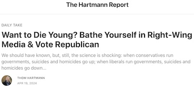She’s pointing here at a report by Thom Hartmann ^[1] on, inter alia, some work she did 10 years ago about the political roots of violent deaths in the US. (Hartmann, not Lee, is the source of the graphic above on bathing in right-wing media.)

I don’t follow Hartmann regularly, but here’s something to understand: he’s definitely a partisan (albeit in favor of my tribe). But his main value to me is not so much the partisan jeremiads so much as the source material he uses. That’s where the real gold is to be found.

So let’s have a look through Hartmann and see what he cites.

Right up front is the conclusion from several papers, in his mildly inflammatory, but admirably clear style:

We should have known, but, still, the science is shocking: when conservatives run governments, suicides and homicides go up; when liberals run governments, suicides and homicides go down.

1: The Australian Study on Suicides

First up is a study from 2002 by Page, Morrell, and Taylor ^[2] which looked at 100 years of data in New South Wales, Australia. They studied suicide rates under Labor and Conservative governments, pretty carefully controlled for confounders, q.v. Their model is a log-rate regression model using government partisanship as one predictor (a rank-ordered 3-level variable for both state & federal conservative, just one, or neither), but also allowing for changes in population age, GDP, drought (indicator variable for a stressor for a pastoral economy), World Wars I and II indicator variables, and an indicator for years during a sedative abuse epidemic:

\[\begin{align*} \ln\left(\frac{n_i}{p_i}\right) &= \beta_1\mathrm{age} + \beta_2\Delta\mathrm{GDP} + \beta_3\mathrm{drought} + \beta_4\mathrm{WW1} + \beta_5\mathrm{WW2} \\ & + \beta_6\mathrm{sedatives} + \beta_7\mathrm{govt} + k \end{align*}\]

Here $n_i$ is the number of suicides in a given year, $p_i$ the corresponding population that year, and $k$ is a background log-rate of suicide independent of the predictor variables.

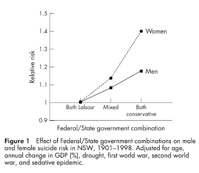Depending on how you slice the population subgroups, the regression is statistically significant at various levels, $p \lt 10^{-3} - 10^{-2}$. The effect size seems to be much stronger on women than on men, as shown here in their Figure 1. It shows how the relative risk ratio for suicide (presumably the exponential of the regression coefficient) increases for mixed or all-conservative government, compared to a labor baseline. The numbers are reported in Table 4:

• Suicide risk:
  • Under mixed governments, suicide risk adjusted for other factors goes up 8% for men and 14% for women.
  • Under pure conservatives, it goes up 17% for men and 40% for women!
• Dose response: The ordering is consistent with risk increase vs amount of conservative government, i.e., consistent with “dose-response” as shown in the graph.

Hartmann reports the BBC’s summary that this led to about 35,000 additional suicides traceable to conservative governments.

(Alas, the data is unpublished as far as I can tell, so I can’t run my own models over this to check. C’est la vie.)

2: The US State-Level Mortality Study, 1999-2019

Inevitably, some American chauvinist will object “but that’s Australia!” as though it were a study of alien beings.

Anent that objection, next up is a study 2022 study by Montez, et al. ^[3] They looked at all-cause mortality, as well as specific associations with cardiovascular disease (CVD), alcohol, drugs, and suicide – the usual sources of “deaths of despair”. ^[4] (Which is, alas, a term your humble Weekend Editor devoutly wishes none of us need ever have heard).

They looked across US states from 1999-2019:

• They used an already well-established methodology for scoring various state polices on a liberal vs conservative continuum.
• They considered 135 state policies, divided into 16 policy domains, of which 8 showed adequate relation to mortality, and sufficient within-state time variation to be able to be modeled. They were: criminal justice, marijuana, environment, gun safety, health and welfare, private labor, economic taxes, and tobacco taxes.
• They considered lag times of 1-5 years for policies to take effect on mortality.
• The modeling was done on a per-gender basis, since as we’ve seen above the policy impacts on men and women can differ greatly.

The regression model was again a log-rate regression model:

\[\log\left(\mbox{age-adjusted mortality rate}\right)_{ij} = \beta_p P_{ij} + \beta_z Z_{ij} + \beta_t T_j + \alpha_i + \mu_{ij}\]

Here index $i$ is for the state, and $j$ is for the year. $P$ is the liberal/conservative score on the policy, $Z$ is a state-level covariate, $T$ is time, $\alpha$ is a background log rate independent of the covariates & time, and $\mu$ is the usual mean-zero error term.

Apparently whatever their statistician told them didn’t survive editing, or got turned into a mush of word salad – so it’s hard to tell a number of things. I think this was a separate regression for each policy $P$, rather than a joint regression that could have studied correlations. Also, the state-level covariates $Z$ are either poorly explained or buried in word salad – one assumes they are things like climate, age, wealth, education, and so on. (This vagueness is, alas, the universal consequence of working with colleagues who are either math phobic or who don’t think it matters much – as I learned to my frustration throughout my career.)

While they report specific associations with CVD and other mortality events, let’s just consider the all-cause mortality result since it is illustrative of the others. This is encapsulated in Figure 2 of the paper, shown here. There’s a lot to unpack in this figure!

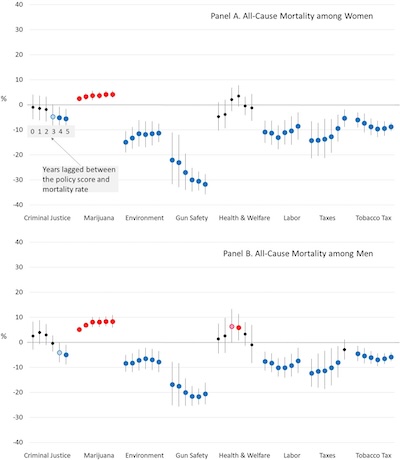
• The 8 policy groups are on the horizontal axis.
• The vertical axis is the percent mortality risk change, scaled to where a state’s liberal/conservative score was a pure 1 or 0. That is, if a state adjusted its policies to one extreme or the other, this is the effect on mortality from the given policy. (I may be somewhat confused on this point.)
• There are 6 dots plotted for each policy, indicating a model with a lag time of 0-5 years to take effect. The whisker is (apparently?) the 90% confidence limit on the change in mortality.
• A dot is black if it didn’t matter much, red if the conservative policy is protective, and blue if the liberal policy is more protective. Light red/blue means $p \sim 0.10$; dark red/blue means $p ~ 0.05$.

Now some interpretation:

• Women (upper panel) and men (lower panel) had broadly similar effects, though sometimes a bit higher or lower. (This is different from the suicide results in Australia, above.) Women, though, were more sensitive to gun safety policy.
• Conservatives win on marijuana policy, by a small but statistically significant amount. (Though I’m not sure why it’s on the positive side of the vertical axis instead of the negative? But this is very clearly what the authors say in the explanatory text, so let’s go with it.)
• Health & welfare are pretty much a wash (possibly due to the national nature of Obamacare overwhelming state-specific policies?).
• Criminal justice is in favor of liberal policies, though only at 3 years lag time or more.
• On all other issues, the mortality risk reduction favors liberal policies. In particular, gun safety is a blowout win for liberal policies, with 20% – 30% mortality reductions.

In the words of the authors, from their abstract (emphasis added):

Especially strong associations were observed between certain domains and specific causes of death: between the gun safety domain and suicide mortality among men, between the labor domain and alcohol-induced mortality, and between both the economic tax and tobacco tax domains and CVD mortality. Simulations indicate that changing all policy domains in all states to a fully liberal orientation might have saved 171,030 lives in 2019, while changing them to a fully conservative orientation might have cost 217,635 lives.

Hundreds of thousands dead: needless, idolatrous sacrifices on the altar of some conservative idée fixe. And this was before the nightmare of conservative resistance to life-saving COVID-19 policies like masking and vaccination, which made everything worse.

(Alas, the data is unpublished as far as I can tell, so I can’t run my own models over this to check. C’est la vie.)

3: US Violent Death Rates vs Presidential Party, 1900 - 2010

Finally we come to the paper of Lee, Wexler, and Gilligan. ^[5] They study violent death rates (basically suicide and homicide) in the US, from 1900 - 2010. They also include some economic variables like GDP and unemployment. The killer analysis here is a $t$-test and a hidden Markov model model time series on whether the president is Republican or Democrat.

It’s admirable to see them use a bit over a century of data, but pretty much impossible to go further. In the 19th century, the roles of the 2 parties were very, very different. In fact, they almost changed places policy-wise: Republicans were the anti-slavery party of the Civil War, as personified by Lincoln; after the Civil War the South consolidated as Democrats while pursuing charming policies like Jim Crow, lynching, and the KKK. That’s pretty much the mirror image of modern times.

They took a different tack, statistically:

• they did some $t$-tests to determine what was associated with presidential party with time lags of 0-2 years,
• then measured correlation controlled for GDP and unemployment.
  The violent death time series is, of course non-stationary (not always draws from the same distribution) and heteroskedastic (time-varying variance). To model this, they used a hidden Markov model (HMM): there’s an underlying finite state machine, in which each state generates a separate time series, and we switch states with a certain probability per unit time. It sounds complicated, but it’s pretty standard for analyzing this sort of time series nowadays.

The looked at annual changes in violent death rates, unemployment, and log GDP.

• The log is necessary in the GDP case because it’s a background exponential growth. The log changes it into linear growth.
• The annual change, rather than absolute rate, removes a linear trend over time, allowing us to focus on changes in rates.

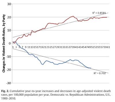For example, consider the annual change in suicide and homicide rates. The null hypothesis here is that this should have no particular trend, since the annual change removes a linear trend and the rate part (divided by the population) makes times with different numbers of people comparable.

If we break that down by Republicans and Democrats and add up the changes year by year, we should expect to see 2 horizontal lines, each with a significant amount of noise making it janky. Sometimes the change will be positive, but that will be canceled by later negative changes. What we see instead is shown here, in the paper’s Figure 2.

• In Republican years, changes are almost always positive, so the cumulative amount fits nicely on a positive-sloped line ($R^2 \sim 86\%$).
• In Democratic years, changes are almost always negative, so the cumulative amount fits nicely on a negative-sloped line ($R^2 \sim 70\%$).

The very high $R^2$ values mean that the party of the president explains 86% or 70% of the variance, i.e., is an incredibly important predictor of changes in suicide/homicide rates.

Now, when modeling a time series of such changes, we have to take into account that it is not stationary, i.e., the parameters of the underlying distribution change over time. And, in fact, the distribution itself can change. So they model this with a finite state machine with probabilistic transitions. Each state generates a stationary time series, but we hop from state to state based on something unobservable, here the “general economic and social health of the nation.”

You might think the optimal HMM would have 2 states: Democratic and Republican. However, when fitting an array of different models using R, the optimum they found was either 3 states (by Bayes Information Criterion) or 4 states (by Akaike Information Criterion and log likelihood). They don’t quite explain their preference for Bayes Information Criterion, but it’s what their Table 4 says.

They assumed transition rates independent of political party for simplicity. However, when testing that addition a 3-state model with slightly better scores on all 3 dimensions (log likelihood, AIC, and BIC). But the difference was small, the states complex to explain, so they abandoned this.

(I’m slightly surprised that there’s not a more modern LASSO-regulated method to fit HMMs? But perhaps there is now, given that the paper is 10 years old.)

The 3-state model is shown here. NB: there are no transitions of significant probability between states 1 & 2, so it’s really a chain, and probably should have been drawn so.

They attempted to explain what each of the states mean, by the ancient and time-honored method of staring at the data and saying “what if…”. Those explanations are shown here also, in their Table 5. This method always seemed like voodoo to me, so I leave you to read Table 5 in peace. (Not that I haven’t stooped to voodoo myself, particularly in explaining factor analyses. But at least I felt bad about it!)

In a way, I’d like to like this paper more than I apparently do.

Of course, the major flaw is not publishing their data and analysis scripts, so I can’t check anything.

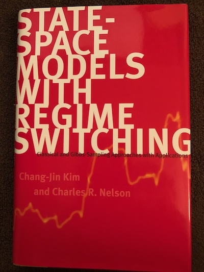Also, everything feels slightly antique. For example, the last time I had to care about non-stationary, heteroskedastic time series was in the early 2000s, to judge by the publication date of the most likely volume on my bookshelf: Kim & Nelson. ^[6] Even back then, though nobody was using LASSO, there were still HMM estimation methods using Kalman filters, Bayesian methods, and Gibbs sampling. It’s a little disappointing not to see any of that here.

Still, none of the authors appear to be deep into statistical modeling. So given that as a Bayesian prior, they did pretty well!

The conclusion is stark. In the words of the authors (first sentence of Section 3, Results):

Suicide, homicide, and combined suicide/homicide rates from 1900 to 2010 were found to be associated with an increase under Republican presidents and a decrease under Democratic ones with statistical significance (Table 1).

(Alas, the data is unpublished as far as I can tell, so I can’t run my own models over this to check. C’est la vie.)

The Weekend Conclusion

These papers are not the only ones. Even on this Crummy Little Blog That Nobody Reads (CLBTNR), we’ve taken a stab at showing this from data, from time to time (here, here, here, here, here, here, here, here, … and that’s not even starting on the partisan nature of vaccine resistance).

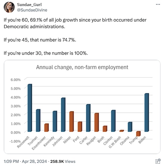
Other people notice, too! Here’s a person pointing out that almost all job growth in recent generations has happened under Democratic administrations:

And patriotism? Don’t get me started. Just listen to the Washington state Republicans saying, “We do not want to be a democracy.” (!) ^[7]

The dangers of general Republican misrule are now clear, from multiple century-long datasets. In the particular person of Trump, it is also associated with his solemn promise to end American democracy. The words of our first president quite well describe Trump, who aspires to be the last president:

“… express your utmost horror and detestation of the Man who wishes, under any specious pretences, to overturn the liberties of our Country, and who wickedly attempts to open the flood Gates of Civil discord, and deluge our rising Empire in Blood.”

– George Washington, “Newburgh Address”, 1783

Republican misrule causes violent deaths, higher unemployment, and lower GDP. This conclusion is not challengable by reasonable people:

• There is over a century of data in support.
• The studies are well-controlled for confounders like world wars and drug epidemics.

If you are an American eligible to vote and you wish to style yourself “pro-life”, then you must vote Democratic, for all offices. Anything else – including 3rd parties, or just not voting – is a vote for more violent deaths, more insurrection, and more economic malaise. Maybe don’t do that?

(Ceterum censeo, Trump incarcerandam esse.)

---

Notes & References

1: Thom Hartmann, “Want to Die Young? Bathe Yourself in Right-Wing Media & Vote Republican”, Hartmann Report, 2024-Apr-19. ↩

2: A Page, S Morrell, and R Taylor, “Suicide and political regime in New South Wales and Australia during the 20th century”, Jnl Epidemiol Community Health vol 56, 766-772, 2002. ↩

3: JK Montez et al., “U.S. state policy contexts and mortality of working-age adults”, PLoS One 17:10 e0275466, 2022-Oct-26. DOI: 10.1371/journal.pone.0275466.

In the interests of full disclosure, we note here that your humble Weekend Editor was briefly a referree for a couple papers in PLoS One, way back in about 2003-2004. ↩

4: Statista Research Department, “Diseases of despair in the U.S. - Statistics & Facts”, Statista, 2024-Jan-08. ↩

5: BX Lee, BE Wexler, and J Gilligan, “Political correlates of violent death rates in the U.S., 1900–2010: Longitudinal and cross-sectional analyses”, Aggression and Violent Behavior, 19:6, 2014-Nov/Dec, pp. 721-728. DOI: 10.1016/j.avb.2014.09.017.

Because this is behind a regrettable paywall, we’ve archived a copy of the paper here, as well as an earlier author’s manuscript here. Perhaps notably, one author on the early copy was removed from the publication copy. No idea what the story was there, but our sympathies to Marilyn Stolar. ↩

6: C-J Kim & CR Nelson, “State-Space Models with Regime Switching”, MIT Press, 1999. DOI: 10.7551/mitpress/6444.003.0015. ↩

7: D Westneat, “The WA GOP put it in writing that they’re not into democracy”, Seattle Times, 2024-Apr-24. ↩