Elections, Fairness Gaps, and Age Gaps

The US is undemocratic in a variety of ways, favoring older voters and very old politicians among them. That might be about to change.

American Un-Democracy

We fail to be a modern democracy in the US in numerous ways. Among them are:

• Unrepresentative Senate: The Senate, at 2 senators per state, fails to represent the population. Instead, it over-represents the large, sparsely populated, rural states which skew heavily red/Republican. Using 2023 population estimates:

  • Wyoming, currently the least populous state, has about 584,000 residents and 2 senators. So they enjoy 1 senator for about every 292,000 people.
  • California, currently the most populous state, has about 38.9 million residents and 2 senators. So they have 1 senator for about every 19,450,000 people.

  In other words, rural, red Wyoming has about 19,450,000 / 292,000 ~ 67 times as much political power per person in the Senate as more urban, blue(ish) California!

• Unrepresentative House: The House, due to the Depression-era Permanent Apportionment Act of 1929, must both have at least 1 representative from each state per the Constitution, but no more than a total of 435. This means – again – the large, sparsely populated, rural states which skew heavily red/Republican are over-represented.

  • Wyoming has 1 representative for 584,000 residents.

  • California has 52 representatives for 38.965 million residents, or 1 representative per 749,300 people.

    In other words: Wyoming enjoys about 749,300 / 584,000 ~ 1.28 times as much political power per person in the House as California.

• Unrepresentative Presidency: The Electoral College is an 18th century Rube Goldberg machine specifically designed for the anti-democratic goal of interposing the judgment of establishment figureheads between the voting populace and the election of a president. (Don’t blame the founders; belief in democracy was a radical step and they took it as far as they could, given their fears as rich, privileged men.)

  It allocates electoral votes to states by the sum of their number of senators and representatives. This, obviously, also over-represents the large, sparsely populated, rural red states. What’s slightly less obvious is that it does so at 2 levels:

  • The number of electoral votes is derived from the number of senators and representatives, already a biased source.

    • Wyoming gets 3 electoral votes for 584,000 people, or about 1 EC vote per 194,666 people.
    • California gets 54 electoral votes, or about 1 EC vote per 720,370 people.

    In other words, Wyoming has about 720,370 / 194,666 ~ 3.7 times the political power per person in presidential elections than California.

  • In case of an Electoral College tie (or if some sociopathic candidate has manged to tie the system in knots), the election is decided by the House. However, each delegation gets 1 vote, i.e., 1 vote per state. This also guarantees control by the low-population rural states, which can out-vote the majority of the population.

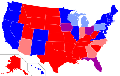    As this map from Wikipedia summarizing the 2008 to 2020 presidential elections shows, there are more red states than blue states. This is a geographic effect: the population results are the opposite. There are far more blue voters, but the red voters are over-represented due to their distribution in rural states.

    But it means, again, over-representation of rural, conservative voters. If an Electoral College tie sends an election to the House, the Republicans will install their candidate regardless of the vote.

• Over-enabling the wealthy: Finally, it costs enormous sums of money to get elected, particularly since the Citizens United and McCutcheon Supreme Court rulings allowed unlimited, secret money from corporations and billionaires. Consequently, our politics favors the extremely conservative interests of the extremely wealthy and the huge corporations.

The last item is of our own creation in modern times.

But it appears that the rest were built in from the beginning of the US, in order to get the slave states to agree. The moral of the story is that if you don’t root out slavers and fascists right down into the ground, they will pollute public discourse for centuries.

Literal centuries, at this point.

Candidate Age Difference & Electoral College Vote Difference

Sadly, all that is just the background. (See up at the top of the page where it says this blog is that of a grumpy old retired scientist? Some days are grumpier than others. The US slide into fascism and racism makes me… grumpy.)

I was reading the venerable blog Crooked Timber (Kant: “Aus so krummem Holze, als woraus der Mensch gemacht ist, kann nichts ganz Gerades gezimmert werden”), and came across an intriguing article by Kevin Munger. ^[1] He’s a political scientist at the European University Institute, in Firenze. Apparently his research interest involves a quantitative view of generational changes in politics, e.g., why the Boomers just won’t go away. ^[2]

Now, I’ve always got a soft spot in my heart for quantitative views of society (or, arguably, a soft spot in my head). His thesis seems to be that:

1. The US is now demographically older than it’s ever been.
2. Younger voter turnout is heavily suppressed in a variety of ways.
3. Younger voters feel that our superannuated politicians do not take their welfare seriously, or even comprehend that there is something to be so taken.
4. Thus there is a lot of voting pressure that would move in favor of younger candidates if any could get through the systemic age blocks in our politics.

Thus Harris is interesting, as a “younger” candidate (at age 60!) who became the nominee by default, in a way that got around all the age blocks.

I’m sympathetic (even as an aging Boomer), but what’s the evidence?

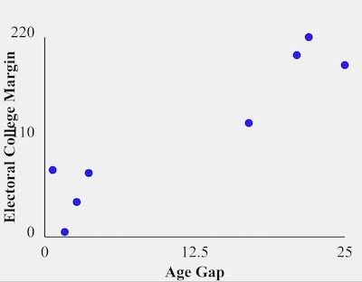Munger gathered data on presidential candidate ages, and their Electoral College votes for 1992-2020. Here he’s plotted the EC vote difference versus the age difference. It looks very much like there are 2 clusters, in which a large age difference leads to a large EC vote difference. However,

• he hasn’t labeled the points by whether the winner was the older or younger candidate (or the Republican vs the Democrat), and
• with only 8 data points one cannot be certain of very much at all!

You know what’s coming next, right?

We’re gonna gather data independently, annotate by who was the winner, test the age gap/EC vote gap hypothesis, and see if it extends to a longer time period. The latter is the most important: lots of things look true briefly, but are of no predictive value since they are artifacts of a limited period of time.

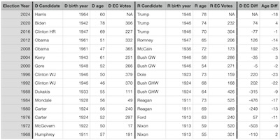So we gathered data from Wikipedia about the ages of US presidential candidates, and US presidential elections by Electoral College margin. We arranged it in a spreadsheet as shown here, in both a binary spreadsheet and a simple tab-separated text file for analysis. ^[3]

Our data runs from 1968 - 2020. We stopped at 1968, because before that the US parties were pretty different animals. The primaries didn’t matter as much, since the candidates were chosen in the proverbial “smoke-filled room” by party czars at the conventions. Only after the 1968 riots and later Watergate did a more democratic primary system take hold.

One thing is immediately apparent by examining the Age Diff column at the far right, where negative numbers mean a younger Democrat and positive numbers indicate a younger Republican: Republicans have never (recently) run a much younger candidate. That is to say, there are no large positive numbers in the last column. Dramatically younger candidates don’t happen often, but when they do, it’s usually Democrats who propose them.

To dive deeper, we wrote an R script ^[4] to explore any relationship between the absolute values of the last 2 columns:

Null Hypothesis: The candidate age difference in absolute value has no influence on the outcome of the Electoral College vote difference in absolute value.

The alternative hypothesis we’ll explore is a dirt-simple ordinary least squares linear regression model with slope $\beta$ and intercept $\alpha$:

This isn’t quite the correct story, since it assumes normally distributed errors around the fitted line, while both variables are bounded below at 0 (because they’re absolute values). There are ways to deal with this, but let’s see if being a bit naïve will get us anywhere.

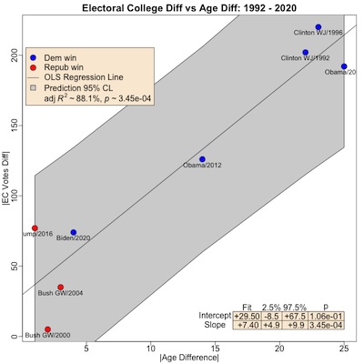
Here’s the result, using 1992 - 2020 data, as Munger did:

Call:
lm(formula = AbsECDiff ~ AbsAgeDiff, data = fitData)

Residuals:
    Min      1Q  Median      3Q     Max 
-39.271 -18.090   1.404  16.311  40.125 

Coefficients:
            Estimate Std. Error t value Pr(>|t|)    
(Intercept)   29.480     15.529   1.898 0.106402    
AbsAgeDiff     7.395      1.017   7.269 0.000345 ***
---
Signif. codes:  0 ‘***’ 0.001 ‘**’ 0.01 ‘*’ 0.05 ‘.’ 0.1 ‘ ’ 1

Residual standard error: 28.04 on 6 degrees of freedom
Multiple R-squared:  0.898,	Adjusted R-squared:  0.881 
F-statistic: 52.84 on 1 and 6 DF,  p-value: 0.0003448

                2.5 %    97.5 %
(Intercept) -8.517304 67.477146
AbsAgeDiff   4.906045  9.884607

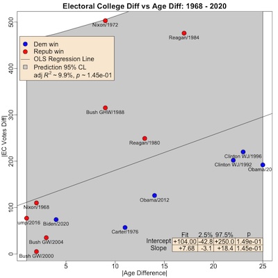
• The horizontal axis is the absolute value of the age difference of the candidates at the time of the election.
• The vertical axis is the absolute value of the difference in their Electoral College votes that resulted from the election.
• Points where the Republican won are red, and points where the Democrat won are in blue. The label just below the point gives the name of the victorious President and the year.
• The black line is the regression line. The gray area around it is the 95% confidence limit on predictions, i.e., error bars if you were to use this model to predict the EC votes.
  • NB: This is one place where ignoring the lower bound of 0 to use a simple least squares model is skating on thin ice; the lower bound of course cannot be negative with absolut value variables!
• The regression is statistically significant with good strength of effect, as reported in the legend in the top left:
  • Statistical Significance: The overall regression has an $F$-statistic with $p \sim 3.45 \times 10^{-4}$, i.e., it’s very unlikely to see data like this if the Null Hypothesis were true.
  • Strength of Effect: The model has an adjusted Pearson $R^2 \sim 88.1\%$, i.e., it predicts a whale of a lot of the variance in the EC vote margin.

The graph agrees with Munger, that a large age difference leads to an EC blowout. The model says you get about 7.4 EC votes per year of age difference, so for Harris’s 18 years younger than Trump we would predict about 29.5 + 18 * 7.4 ~ 163 more EC votes for Harris.

However:

• With only 8 data points, we can’t really trust it.
• All the effect is due to Obama and the earlier Clinton elections. Without those, the effect goes away.

So now let’s look at it with a somewhat longer baseline, from 1968 - 2020.

Call:
lm(formula = AbsECDiff ~ AbsAgeDiff, data = fitData)

Residuals:
    Min      1Q  Median      3Q     Max 
-131.09  -90.04  -60.29   31.91  330.26 

Coefficients:
            Estimate Std. Error t value Pr(>|t|)
(Intercept)  103.656     67.237   1.542    0.149
AbsAgeDiff     7.676      4.925   1.559    0.145

Residual standard error: 147.2 on 12 degrees of freedom
Multiple R-squared:  0.1683,	Adjusted R-squared:  0.09904 
F-statistic: 2.429 on 1 and 12 DF,  p-value: 0.1451

                 2.5 %    97.5 %
(Intercept) -42.841228 250.15248
AbsAgeDiff   -3.055107  18.40764

Here we see that the effect goes away. The model is not statistically significant ($p \sim 0.145$), nor does it predict much of the variance ($R^2 \sim 9.9\%$). The gray band, the prediction 95% confidence interval, covers almost everything, indicating we really can’t predict anything.

In professional statistician’s language: we got nuthin’.

We note a few enticing details:

• The effect is ruined by 4 Republican victories by Reagan, Nixon, and the elder Bush. These were “blowout” EC vote totals, but middling age differences.
• Other than Biden, every Democratic win has been by a much younger candidate.
• The slope coefficient, while not statistically significant, is still about 7.5 Electoral College votes per year of age difference. Probably not a meaningful thing?

You can come up with arguments for discarding the data before 1992. But… throwing out inconvenient data that invalidates your theory is not a way to earn your statistician’s respect.

We’re left with the idea that either the age difference predicting an Electoral College blowout is a recent phenomenon, or actually false when we see enough data.

What About Walz?

People have been looking at these pictures of Harris and Walz, wondering why she picked such an older running mate. In fact: they are the same age.

How can that be?

There could be some genetics in play, but really the obvious answers apply:

• Men tend to lose hair with age more than women.
• Women are more likely to dye hair to erase gray.
• Also women are more likely to moisturize, and that probably shows.

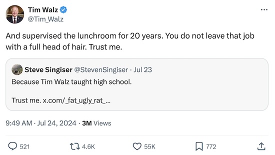
True to his sense of humor, though, Walz saw this and said he only looks old, it’s the stress from decades of supervising a high school lunchroom:

I believe him!

High school, especially including the cafeteria, was bad enough even just for a couple years as a student. To cope for decades with a roomful of teenage angst and BS is truly a labor of Augean scale.

Funding & Demographic Differences

Back to Munger: whether or not the EC vote difference is a result of age differences, there have been other material changes in the election with the advent of Harris.

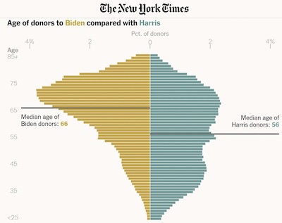Munger shows a bidistribution plot from the New York Times of what age groups are donating.

• Notably, Biden’s donors were quite old: median age 66 years old, and modal age around 70 years old.
• However, Harris’s donors appear to be much more evenly spread across ages. Yes, the median is 56 years old, but look at the breadth: almost evenly spread from 35 - 65.

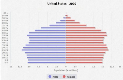Another important point is to compare this to the age distribution of the whole population, a fortiori the voting population in the US. It’s shown here for men and women.

• Biden’s main donors, modal age early 70’s, are on the declining side of population prevalence: there just aren’t as many of them to vote for him.
• Harris’s donors, on the other hand, at 35 - 65, reflect the broad population as a whole and thus, we hope, votes available to her.

Donations still skew older, though “that’s where the money is” as Willie Sutton is supposed to have said.

The Weekend Conclusion

As you can see here, even among Weekend Publishing’s management clade, the young are watching even as the elders snooze.

Alas, as non-citizen cats, they are ineligible to vote. They reassure me, however, that they favor Harris/Walz. And that I should do so as well, under penalty of claw.

Munger concludes (emphasis mine):

The implicit prediction of this article is that Harris will win in a landslide. I don’t believe my 8-point scatter plot enough to go so hard against conventional wisdom. But so far, the evidence points to an unmet demand for younger politicians appealing to younger voters.

The data are slim, but somehow they feel like a persuasive summary of the zeitgeist: our younger (also browner, queerer, poorer) co-citizens want to shove the conservative legacy of their elders out of the way. They want what I want: the good things available other developed nations like universal health care, strict federal gun control, accessible & cheap mass transit, less intrusive government, unions, less economic inequality, easy access to education, comfortable retirements…

As practically nobody says anymore (at least not in Latin, outside certain obscure novels and difficult-to-find clocks): Dum vivimus, vivamus.

Basically, we just want to live.

(Ceterum censeo, Trump incarcerandam esse.)

Addendum 2024-Sep-09: Just From Carter Onwards?

After brief but pleasant email exchange with Munger on period dependence, I decided to try just from 1976-2020. This is because, after Nixon, the American political parties changed fairly dramatically.

• Before that, primaries were mostly a way of taking the electorate’s temperature in a non-binding way. Party conventions were a time for the party bosses to get together, choose a nominee in the proverbial smoke-filled back room, and then direct the delegates under their control to cast show ballots accordingly.
• After that, the primaries became binding. (Mostly: there are still vestiges of the old system with “super-delegates”, who are party officials and elected politicians who still get to cast votes not bound by the primaries.) I remember seeing in 1976 the anger and angst of Kennedy delegates at the Democratic convention, over being “robots” who would have to nominate Carter.

So let’s remove Nixon. (And who doesn’t wanna do that?!) Here’s the result with just data from 1976-2020:

Call:
lm(formula = AbsECDiff ~ AbsAgeDiff, data = fitData)

Residuals:
    Min      1Q  Median      3Q     Max 
-103.19  -64.44  -50.31   21.46  262.96 

Coefficients:
            Estimate Std. Error t value Pr(>|t|)  
(Intercept)   63.307     61.075   1.037    0.324  
AbsAgeDiff     8.808      4.211   2.091    0.063 .
---
Signif. codes:  0 ‘***’ 0.001 ‘**’ 0.01 ‘*’ 0.05 ‘.’ 0.1 ‘ ’ 1

Residual standard error: 118.8 on 10 degrees of freedom
Multiple R-squared:  0.3043,	Adjusted R-squared:  0.2347 
F-statistic: 4.374 on 1 and 10 DF,  p-value: 0.06297

                  2.5 %   97.5 %
(Intercept) -72.7770500 199.3901
AbsAgeDiff   -0.5754264  18.1910

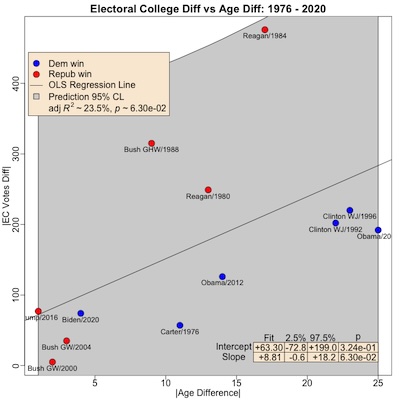It helps to remove Nixon, but only a little bit: marginally not statistically significant with $p \sim 6.3\%$, and only marginal strength of effect in terms of variance explained with Pearson $R^2 \sim 23\%$.

It removes the 1972 Nixon blowout where he won, as I recall, every state but Massachusetts and 1 faithless elector vote in Virginia. However, it also removes the Nixon 1968 data point, which was low age difference, low Electoral College vote difference, and pretty much on the model prediction line.

What still kills the model are the GHW Bush blowout and the 2 Reagan blowouts. It’s pretty hard (for me, at least) to come up with an excuse to remove those from the data.

Notes & References

1: K Munger, “The (Electoral) Politics of Age Gaps”, the venerable Crooked Timber blog, 2024-Aug-28. ↩

2: K Munger, Generation Gap: Why the Baby Boomers Still Dominate American Politics and Culture, Columbia University Press, 2022. ISBN-13: 978-0231200875. ↩

3: Weekend Editor, “Dataset of presidential candidate ages and electoral vote counts”, Some Weekend Reading blog, 2024-Sep-06.

NB: These data are also available as a spreadsheet in Apple Numbers format. ↩

4: Weekend Editor, “R script to analyze dataset of presidential candidate ages and electoral vote counts”, Some Weekend Reading blog, 2024-Sep-06.

NB: There is also available a text transcript of running this, to cross-check with the plots. ↩