US Political Parties and the Budget Deficit

Previously, we looked at the party control of the 3 US government branches and their effect on the economy. We unaccountably left out the budget deficit, so let’s have a look at that: Republicans are commonly thought to be good for the budget, but are they really?

The Budget Data

We’re really just redoing the analysis that previously told us Republicans were bad for unemployment (U6) and inflation (CPI-U). ^[1]

Now let’s look at the budget deficit. We’ll look at the deficit itself, as well as the deficit as a percent of GDP, to account for economic growth. As before, we’ll look at the era from 1977 to the present, since before 1977 US politics (especially Republican politics) looked quite different.

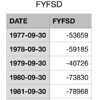
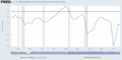
• Budget surplus/deficit: Here we used the time series FYFSD, from the FRED databases of the St. Louis Fed. ^[2] It reports the annual federal government’s budget deficit (negative) or surplus (positive), in millions of dollars. (Yes, there were some years of budget surplus under Clinton in the late 90s.) It looks as shown here, reported on Sept 30 of each year since that’s the federal fiscal year-end. The collected data run 1977 - 2023.

  As before, we combine 2 years by adding together the deficits, to get a composite figure for each congressional term. Then we compare this to the previous congressional term, and annotate a term as “Better” if the deficit was a less negative number, or “Worse” if the deficit went further negative. This gives us an idea of whether the policies of that term moved the budget needle or not, in raw dollar terms.

  Since these figures are (a) over short time spans and (b) relative to the previous term, we don’t need to correct for inflation.

• Budget surplus/deficit as a % of GDP: But even if we don’t need to correct for inflation, it may make sense to correct for the size of the GDP, which does, after all, grow! We should be less worried about a deficit if the economy is dramatically larger. There is also a counter-cyclical effect, where the deficit grows in times of recession due to falls in income and hence government tax revenue.

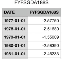
  To do this, we used the time series FYFSGDA188S, also from the FRED databases of the St. Louis Fed. ^[3] It takes the annual deficit data in the FYFSD series, and combines them with the GDP series GDPA ^[4], in the following way:

  \[\mbox{FYFSGDA188S} = \frac{\mbox{FYFSD} / 1000}{\mbox{GDPA}} \times 100\]

  The factor of 1000 is because FYFSD is reported in millions, while GDPA is reported in billions and those are a factor of 1000 different. The final factor of 100 is to report the ratio as a percentage. (We did not do this calculation ourselves, but accepted the FRED database’s version of it. No need to check the Fed’s arithmetic!)

  The collected data here also run 1977 - 2023.

  Then, when combining years into a figure for a 2-year congressional term, we add the percentages. Thus for a congressional term, the max would be a 200% figure.

All these datasets were loaded, transformed into Better/Worse binaries, and joined with the partisanship data from the previous analysis by a new R script analogous to the previous one. ^[5]

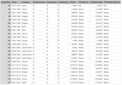The composite dataset it constructs, consisting of years, congressional terms, partisan ship of House/Senate/Presidency, deficit data, and binarization to Better/Worse, is also available as a tab-separated text file for inspection. ^[6] It is also shown here in all its glory.

(NB: “All its glory” is, of course, self-directed sarcasm. There are only 23 data points, so not enough to do cross-validation and L1 LASSO regularization, which are kind of the bare minimum. This analysis is exploratory, at best.)

(NB: Also, the indicator variables are “NA” for 1977, since they are based on a change with respect to the previous year. We’ve elected here to chop of the data at 1977 since before that we’re into Nixon and a different world. We could, perhaps, have included 1976 just for purposes of the first year’s difference, but we didn’t do that.)

Analyses, or Why Jumping to Conclusions is Silly & Dangerous

As before, we performed a logistic regression using both the deficit and deficit as a percent of GDP, predicting from the partisanship of the 3 branches of the federal government:

Here, the R regression software glm() took the D level of each variable as the base, and the R level as the contrast with respect to that baseline. What this means is that a positive regression coefficient will mean that Republicans in that branch are generally bad; a negative regression coefficient will mean Democrats in that branch are generally bad.

Also as before, we did not attempt to include interaction terms to account for when one party has more than 1 branch under its control. The power of a trifecta is certainly real, but that ends up being an 8-parameter model which we simply cannot fit with only 23 data points!

Since we don’t have the data to crossvalidate, we’ll again be satisfied with:

• We’ll assess the statistical significance of the fits with the Akaike Information Criterion (AIC). This is a penalized log-likelihood measure, in which models with more parameters are penalized and thus have to achieve better log likelihoods. The preferred model has the smaller AIC. This will permit us to compare the 4- and 8-parameter models above on an even basis. It is also as close as we can come to fighting over-fitting, without enough data to power LASSO.

  It will not, however, tell us a significance cutoff threshold. That’s ok, we’re not crossvalidating due to lack of data anyway.

• To assess the strength of the model, we’ll run each regression model on its own training data (A cardinal sin! Or at least an ordinal sin?). That will give us a probability of “Worse” for each congressional term. We’ll sort by that probability, and then do a Mann-Whitney rank test to see if the Worse/Better outcomes are statistically significantly sorted.

  That is to say, a significant Mann-Whitney $p$-value will mean at least we can predict well on our own training set. If we can’t even do that, the model is nonsense. If we can, it might mean something, but we don’t have the data to crossvalidate.

The Deficit Itself

Here’s the result of the logistic regression for the deficit:

Coefficients:
                 Estimate Std. Error z value Pr(>|z|)  
(Intercept)      0.396021   0.941318   0.421   0.6740  
PartyPresidentR  2.577359   1.337714   1.927   0.0540 .  
PartyHouseR     -2.570177   1.475261  -1.742   0.0815 .   
PartySenateR    -0.009574   1.540517  -0.006   0.9950  
---
Signif. codes:  0 ‘***’ 0.001 ‘**’ 0.01 ‘*’ 0.05 ‘.’ 0.1 ‘ ’ 1

(Dispersion parameter for binomial family taken to be 1)

    Null deviance: 29.767  on 21  degrees of freedom
Residual deviance: 17.846  on 18  degrees of freedom
AIC: 25.846

Number of Fisher Scoring iterations: 5

This says a Republican president is bad news, but a Democratic House is also bad news. Both of those are just marginally below statistical significance with $t$-test $p$-values of 5.4% and 8.1%, respectively. The Senate is more or less irrelevant.

Does it predict much of anything? Let’s use the model to compute $\hat{p}$, the model’s probability that things will get worse. Sort by that, and then do a Mann-Whitney test to see if Better/Worse are enriched at the top/bottom of the list.

The result looks like this, with Mann-Whitney very significant at $p \sim 0.0045$:

       Years PartyPresident PartyHouse PartySenate DepVar      pHat
5  1995-1996              D          R           R Better 0.1012211
6  1997-1998              D          R           R Better 0.1012211
7  1999-2000              D          R           R Better 0.1012211
15 2015-2016              D          R           R Better 0.1012211
13 2011-2012              D          R           D Better 0.1020954
14 2013-2014              D          R           D Better 0.1020954
9  2003-2004              R          R           R  Worse 0.5971560
10 2005-2006              R          R           R Better 0.5971560
16 2017-2018              R          R           R  Worse 0.5971560
20 1979-1980              D          D           D  Worse 0.5977312
4  1993-1994              D          D           D Better 0.5977312
12 2009-2010              D          D           D  Worse 0.5977312
18 2021-2022              D          D           D  Worse 0.5977312
8  2001-2002              R          R           D  Worse 0.5994569
21 1981-1982              R          D           R  Worse 0.9509119
22 1983-1984              R          D           R  Worse 0.9509119
23 1985-1986              R          D           R  Worse 0.9509119
17 2019-2020              R          D           R  Worse 0.9509119
1  1987-1988              R          D           D Better 0.9513569
2  1989-1990              R          D           D  Worse 0.9513569
3  1991-1992              R          D           D  Worse 0.9513569
11 2007-2008              R          D           D  Worse 0.9513569

Note that, as we interpreted above, the R values are enriched at the bottom (Worse) end of the presidency column, but the D values are at the bottom of the House column. The Senate column is mixed.

Conclusion: We have exploratory (non-crossvalidated, non-regularized, underpowered) evidence that Republicans are bad in the Presidency, but Democrats are bad in the House, and that the Senate doesn’t matter.

The Deficit as a % of GDP

Now let’s repeat that analysis using the deficit as a % of the GDP as the variable being predicted:

Coefficients:
                Estimate Std. Error z value Pr(>|z|)  
(Intercept)     -2.01936    1.22494  -1.649   0.0992 .
PartyPresidentR  2.80601    1.28211   2.189   0.0286 *
PartyHouseR     -0.33920    1.17607  -0.288   0.7730  
PartySenateR     0.04027    1.16236   0.035   0.9724  
---
Signif. codes:  0 ‘***’ 0.001 ‘**’ 0.01 ‘*’ 0.05 ‘.’ 0.1 ‘ ’ 1

(Dispersion parameter for binomial family taken to be 1)

    Null deviance: 29.767  on 21  degrees of freedom
Residual deviance: 21.690  on 18  degrees of freedom
AIC: 29.69

Number of Fisher Scoring iterations: 4

Again the presidency is significant, with Republicans there being bad, and statistically significant with $p \sim 2.9\%$. However, neither the House nor the Senate are statistically significant ($p \sim 77\%$ and $p \sim 97\%$, respectively).

Doing the same trick as above, making predictions via the logistic regression $\hat{p}$, sorting, and doing Mann-Whitney we also get a statistically significant prediction at $p \sim 0.015$:

       Years PartyPresident PartyHouse PartySenate DepVar       pHat
13 2011-2012              D          R           D Better 0.08638853
14 2013-2014              D          R           D Better 0.08638853
5  1995-1996              D          R           R Better 0.08962004
6  1997-1998              D          R           R Better 0.08962004
7  1999-2000              D          R           R Better 0.08962004
15 2015-2016              D          R           R Better 0.08962004
20 1979-1980              D          D           D Better 0.11718570
4  1993-1994              D          D           D Better 0.11718570
12 2009-2010              D          D           D  Worse 0.11718570
18 2021-2022              D          D           D Better 0.11718570
8  2001-2002              R          R           D  Worse 0.61003387
9  2003-2004              R          R           R  Worse 0.61956964
10 2005-2006              R          R           R Better 0.61956964
16 2017-2018              R          R           R  Worse 0.61956964
1  1987-1988              R          D           D Better 0.68711157
2  1989-1990              R          D           D  Worse 0.68711157
3  1991-1992              R          D           D  Worse 0.68711157
11 2007-2008              R          D           D Better 0.68711157
21 1981-1982              R          D           R  Worse 0.69570273
22 1983-1984              R          D           R  Worse 0.69570273
23 1985-1986              R          D           R Better 0.69570273
17 2019-2020              R          D           R  Worse 0.69570273

Consistent with our interpretation from the regression coefficients, the Presidency column is enriched with R’s at the bottom/Worse end. The House and Senate are mixed.

Conclusion: We have exploratory (non-crossvalidated, non-regularized, underpowered) evidence that Republicans are bad in the Presidency, and that the House and Senate don’t matter much.

Summary

The fit of the raw deficit is slightly better quality (lower AIC), and slightly more Mann-Whitney significant in predicting. On the other hand, the deficit/GDP model includes important information about the growth of the economy over the period studied. Also, the Presidency regression coefficient when using GDP is statistically significant, whereas none of the coefficients are when just using GDP.

In either case, they agree that Republican Presidents are bad. They differ as to whether Democrats in the House matter or not. Neither model cares about the Senate.

The Weekend Conclusion

1. Republican presidents are bad news for the deficit, whether by itself or as a percent of GDP.
2. Other branches and whether Democrats occupy them are arguable either way, at least according to this rather small dataset that couldn’t be cross-validated or LASSO regularized.

(Ceterum censeo, Trump incarcerandam esse.)

Notes & References

1: Weekend Editor, “US Political Parties and the Economy”, Some Weekend Reading blog, 2024-Oct-28. We will be re-using the script from this post for this analysis. ↩

2: St. Louis Fed Staff, “Federal Surplus or Deficit (FYFSD)”, FRED databases, US Federal Reserve Bank of St Louis, data from 1977 – 2023 retrieved 2024-Dec-04. A local copy is archived here for peer review purposes. ↩

3: St. Louis Fed Staff, “Federal Surplus or Deficit - as Percent of Gross Domestic Product (FYFSGDA188S)”, FRED databases, US Federal Reserve Bank of St Louis, data from 1977 – 2023 retrieved 2024-Dec-04. A local copy is archived here for peer review purposes. ↩

4: St. Louis Fed Staff, “Gross Domestic Product”, US Federal Reserve Bank of St Louis, data from 1977 – 2023 retrieved 2024-Dec-04. ↩

5: Weekend Editor, “R script to analyze partisanship of government branches and budget deficit”, Some Weekend Reading blog, 2024-Dec-05.

There is also available a text transcript of running this script, so you can check that it says what I say it says.↩

6: Weekend Editor, “Consolidated Congressional Term Dataset of Partisanship of Federal Government Branches and Economic Results, 1977-2023”, Some Weekend Reading blog, 2024-Dec-05. ↩